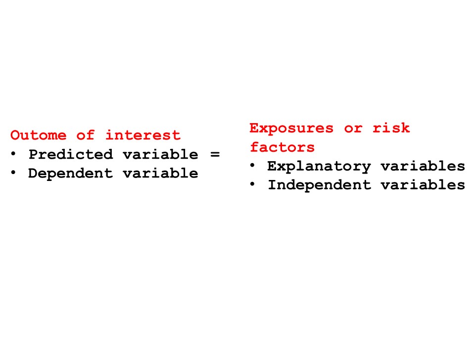
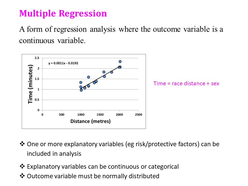
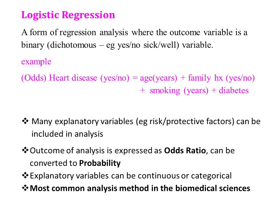
These remarks apply to both a ‘standard’ negative binomial regression and a ‘zero truncated’ negative binomial regression. A zero truncated negative binomial regression is appropriate when there are no zero values, for example if you are counting days in hospital. In the current example, our outcome variable is number of hours on a ventilator. Explanatory variables are Apache Score (a measure of disease severity) and sex.
The negative binomial regression model will output either a standard set of coefficients or an exponentiated set of coefficients, which reflect the IRR. You will see a coefficient for each of the explanatory variables in the model, and a coefficient for the constant term.
The IRR is the exponential of the coefficient, not the log of the coefficient. Remember it is NOT a linear regression, but a (zero truncated) negative binomial regression. Two different kinds of regression.
Incidence rate ratio: the rate
The ‘rate’ part comes in because the outcome variable is actually a count, in this case a count of ventilation hours. We really mean it is a count of ventilation hours per person.
Contrast this with another scenario where you are looking at aircraft flight delays over a number of different airlines. You can’t just talk about the number (count) of flight delays, you have to take into account the number of flights a particular airline may have scheduled. Five flight delays out of ten scheduled flights would be terrible, whereas five flight delays out of 500 flights would not be too bad. With this kind of data you enter the ‘exposure’ variable (number of scheduled flights) as what is called an ‘offset’ variable into the regression equation.
But in our current example, we are talking about ventilation hours per one person, so we don’t have to include an offset.
Incidence rate ratio: the ratio
Look at the attached Microsoft Excel spreadsheet
to see how the ratio part works. Here I used an example where we had ventilation hours as the outcome variable with two predictors, apache3 (Apache III score, a numeric indication of the severity of illness, higher is worse) and sex (male=0, female=1). The IRR for apache3 is 1.0035. This is equal to e^0.0035, the coefficient for the neg bin equation.
The IRR is the ratio of the ventilation hours at a given level of apache3 (say 101) divided by the predicted ventilation hours at an apache3 score of 1 unit less (say 100), holding sex constant. It’s easier to see this if you look at row 15 of the spreadsheet – at apache3=101, ventilation hours = 50.07, at apache3=100, ventilation hours = 49.9.
50.07/49.9 = 1.0035, the ‘incidence ratio’ of ‘new’ hours on a ventilator. You can see this holds true for any value of ventilation hours.
The negative binomial equation is:
loge (ventilation hours) = intercept+ b1* apache3+ b2*sex
= 3.56 + 0.0035*apache3+ 0.18*sex
– see the first set of rows on the spreadsheet
The negative binomial equation with IRR as the output is:
ventilation hours = exp(intercept) * exp(b1*apache3) * exp(b2*sex)
= exp(3.56) * exp(0.0035*apache3) * exp(0.18*sex)
– see the second set of rows in the spreadsheet
Have a play with the spreadsheet inputting different values for apache3 and sex. You could use this with your own equations to see the predicted outcome measure of your own interest.
