Introduction

Here we’ll take a brief, but hopefully practical, overview of sampling in the context of designing a research project, and how to select a suitable sample size.

The participants you include in your study are an important consideration, to ensure that the results of your study can be extended or generalised to a larger group than your actual study participants. This is known as ‘generalisability’, or ‘external validity’.

Sample size is important to make sure that you include enough subjects to have a reasonable chance of detecting a difference between groups, for example difference in response rates to a new treatment compared with an old treatment, if there is one, and that you do not unnecessarily include too many subjects which might be unethical or an unjustifiable use of scarce research funding or resources. Having said that, a larger group is usually very desirable to improve the precision of the findings of your study and enable more detailed analyses to be run.

Study protocols and ethics applications invariably require a justification for sample size.

What is a sample?

If we want to know the exact ‘truth’ of something, we can measure every person (or item) in a whole population. This is a ‘census’ – ‘a study that involves the observation of every member of a population’. Measuring an entire population, for example in the periodic Australian census, is expensive and inconvenient, and not usually feasible in the context of medical research.

Instead we select a much smaller number of subjects who we hope are representative of the population we’d like to study.

We assume that this reflects the population, and that the results are estimates of the ‘truth’. Hence, summary statistics such as mean, median or proportion are given with standard deviation, standard error or a confidence interval, to indicate the precision of our estimate.¹

We do a research study, in the biomedical or veterinary context, in order to apply the result to some ‘target population’. For example, if you are a respiratory clinician, you might like to know whether dornase alfa administered to children and adolescents aged 5 – 18 with cystic fibrosis was effective in improving lung function in this group.

The target population in this example is ‘children and adolescents aged 5 – 18 with cystic fibrosis’. It is self-evident that it would not be feasible to test the drug in ALL people with cystic fibrosis aged 5 – 18 in the world; however we would like to apply the results to this group in general. Thus, the research needs to be conducted in a group which represents all people with cystic fibrosis aged 5 – 18 years.

The research process can be pictured as an idea, followed by development of a structured research question, typically along the PICO guideline of Population, Intervention, Comparator. This is followed by development of specific statistically tested hypothesis or hypotheses. We then go ahead and conduct out study, think about our results and draw our conclusions.

 

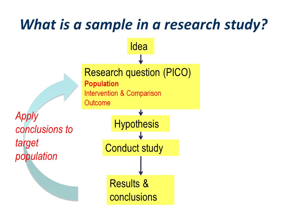
Hopefully, the conclusions will be applied to our original wider population of interest. This is the essence of the process of translation of research into practice.

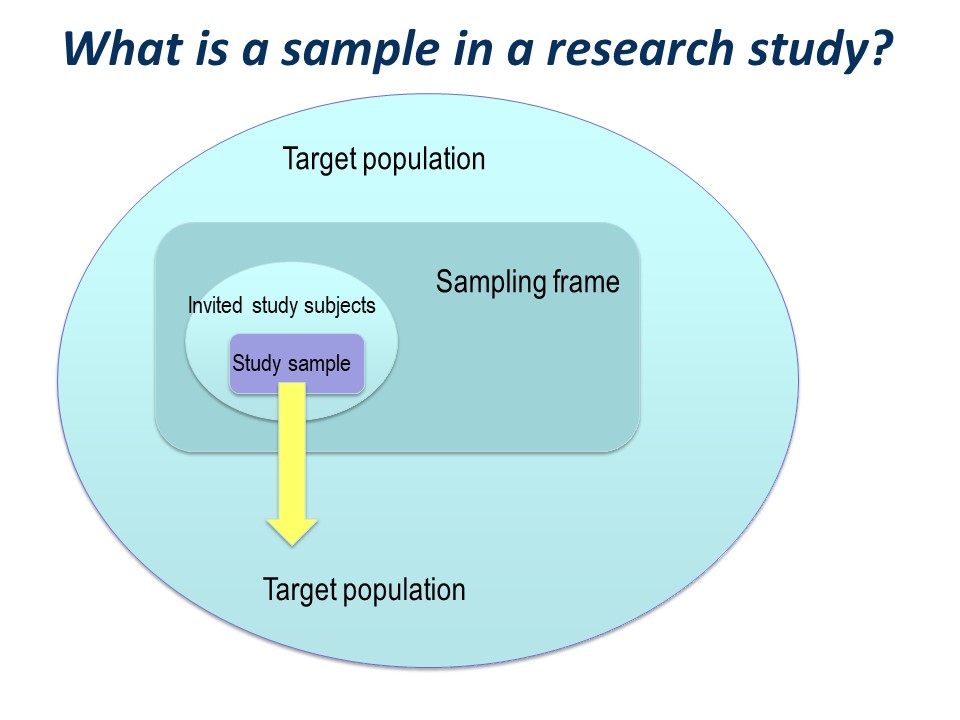
There is a big ‘step down’ from the target population to the actual study sample. It is very useful to conceptualise this using a diagram like this on – you can see how important the selection of the study sample is.

You have a large ‘target population’, the population to which you wish to apply the conclusions of your study.

Everitt defines a target population as

‘The collection of individuals, items, measurements, etc. about which is is required to make inferences. Often the population actually sampled differs from the target population, and this may result in misleading conclusions being made’. ¹

The sampling frame

Then you have a ‘sampling frame’. This is the group of subjects to which you have access – essentially a list – from which you hope to select your study sample.

It could be quite specific, for example, you may have an actual list of all the patients in your clinic. You may have a list for potential control subjects.

It might be less specific; you may not have a list of patients in your clinic, but plan just to invite everyone who comes to clinic over a specified time period, say 3 months or 6 months.

It may not be practical to invite every single person in your sampling frame to participate in the study. For example, if you are recruiting over a 3 month time period, those attending over the other nine months of the year will not be invited. Thus, not everyone in the sampling frame is likely to be invited to participate in your study.

You might have a list of 6,000 people from whom to select your study subjects – it is not practical to invite all of them to participate in your study.

So the invited study subjects are a subset of the sampling frame. (See selecting a random sample in later slides).

The study sample

Of those who are invited to participate, not all will agree or consent to being part of your study. So in turn, the initial study sample will be a subset of the invited subjects.

Finally, of those people who consent to participate in your study, some may prove ineligible for the study, if there is any kind of screening for eligibility, and some are likely to drop out.

The subjects left at the end of the study, for whom outcome information is available, constitute the final study sample.

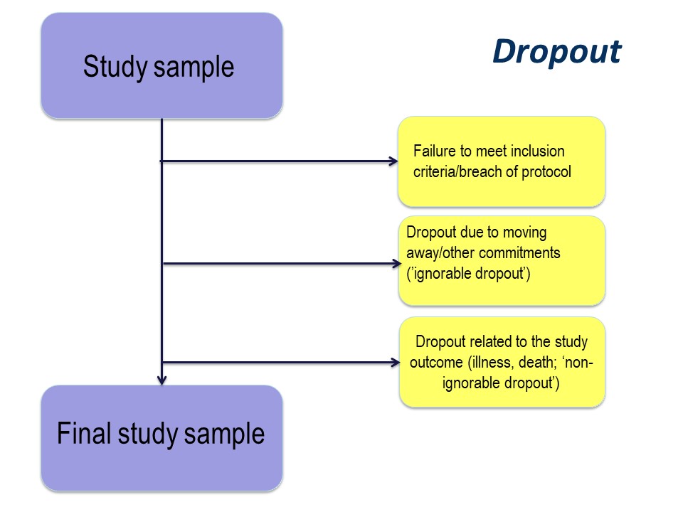
Dropout

The reason for drop out is important. Participants may drop out of studies because of simply electing not to continue with a study, by moving away, or because of illness or death.

Any study dropout is undesirable, but drop out because of illness or death must be taken into account in the statistical analysis. For example, in our cystic fibrosis example, the study was conducted over 96 month. If, hypothetically, some had dropped out because of illness (with very poor lung function) or death, especially if there were more dropouts in the active treatment group, those surviving until the end of the study will be those with the best lung function. This might produce a spurious ‘result’ of improved lung function in the treatment group.

The importance of the reason for dropout will vary depending on the nature of the research that you are doing, but it is very important to consider the implications of dropout at the study design stage.

Summary and practical example – target population to study sample

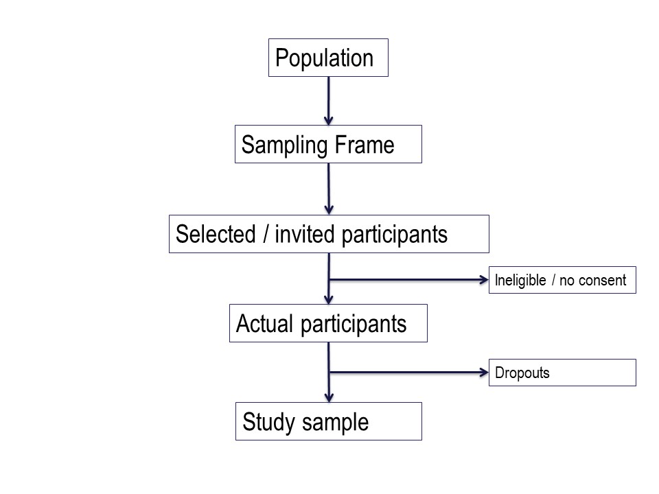
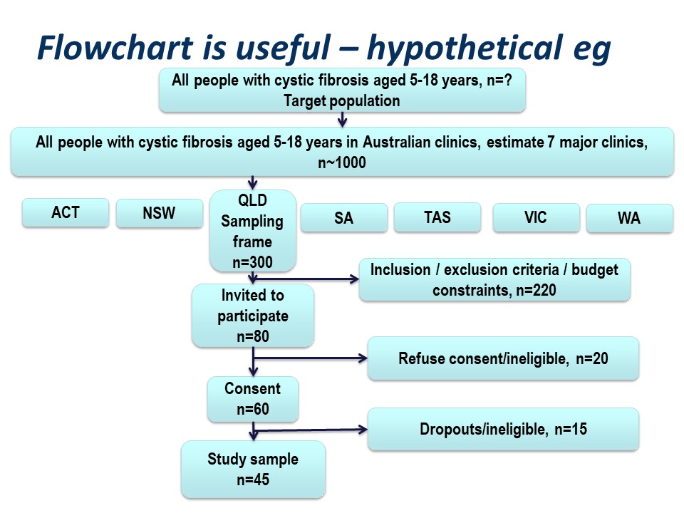
Figure 4 below is a summary of the population to which the study results are intended to be applied, and the flow of patients through a study. Note that essentially all of the ‘standards of reporting’ such as CONSORT .²and STROBE,³ by which editors and reviewers are guided, strongly recommend the use of a flowchart in your manuscript. If you are writing a Cochrane Review a flowchart is essential.⁴

Hypothetically, suppose we want to run a trial of some drug, or an observational study, in people with cystic fibrosis. We want our conclusions to be applicable to all people with cystic fibrosis. We are based in Queensland and have access to patients of the Queensland clinic. Are our potential study subjects representative of all people with CF?

Consider the flow of subjects through the study. We are restricted by feasibility to the Queensland clinics, probably restricted to the Brisbane clinic. This might give us a sampling frame of 300 people. From this, we consider the inclusion and exclusion criteria, which will render a proportion of subjects ineligible for the study at this step. Additionally, we may have budgetary constraints that limits the number of subjects we can include in the study. We have to ‘guestimate’ the likely study sample, the potential dropouts to the study, and work backwards to invite a suitable number of participants. Let’s say we invite 80 people to participate.

Of those invited to participate, not all will consent. Some patients will be found to be ineligible during the patient information step of obtaining informed consent. Here, we have 20 patients who either refuse consent or are ineligible when we initially invite them to participate.

Additionally, sometimes it is not possible to assess subjects for eligibility before consent, for example if some screening test, like a blood test, needs to be applied. In this hypothetical example, we lost some subjects who are ineligible at this point, and others who may drop out for reasons either unrelated or related to the study. We lose another 15 subjects here.

Thus our final study sample is 45 people (Figure 5).

What sample size do I need to select?

This brings us nicely to the topic of sample size – ‘how many subjects do we need in our study’, because the statistical analysis will be performed on the study sample, i.e. those subjects who have actually participated in the study.

Estimates and measures of uncertainty

To expand a little on estimates and confidence intervals:

Any statistic (mean, median, proportion) calculated from the study sample is only an estimate of the ‘true’ statistic we would get if we measured every person in the target population

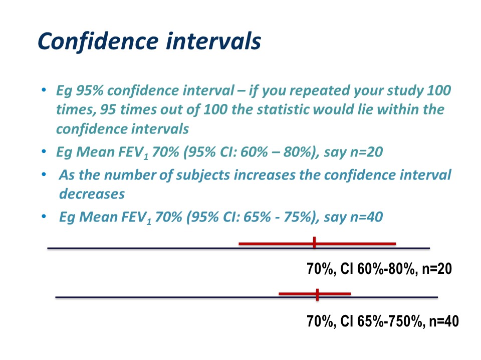
If we started again and selected a different sample, we would get a slightly different statistic. For this reason, statistics calculated from samples should be reported with a confidence interval. For a 95% confidence interval – if you repeated your study 100 times, 95 times out of 100 the statistic would lie within the confidence intervals.^5-7

For example for 20 subjects, the mean FEV₁ and 95% confidence interval might be 60% – 80%. As the number of subjects increases the confidence interval decreases. If you measured 40 subjects, the mean FEV₁ might still be 70% or something close to it, but the confidence interval would be narrower, say 65% – 75%.

Clustering

Valid conclusions assume that the study sample constitutes a random sample. Everitt¹ defines a random sample as:

‘….a sample of n individuals selected from a population in such a say that each sample of the same size is equally likely’. ¹

For example, in the diagram, if the blue circle represents the sampling frame, and the red dots represent subjects in your study, your comparisons assume the first picture, not the second.

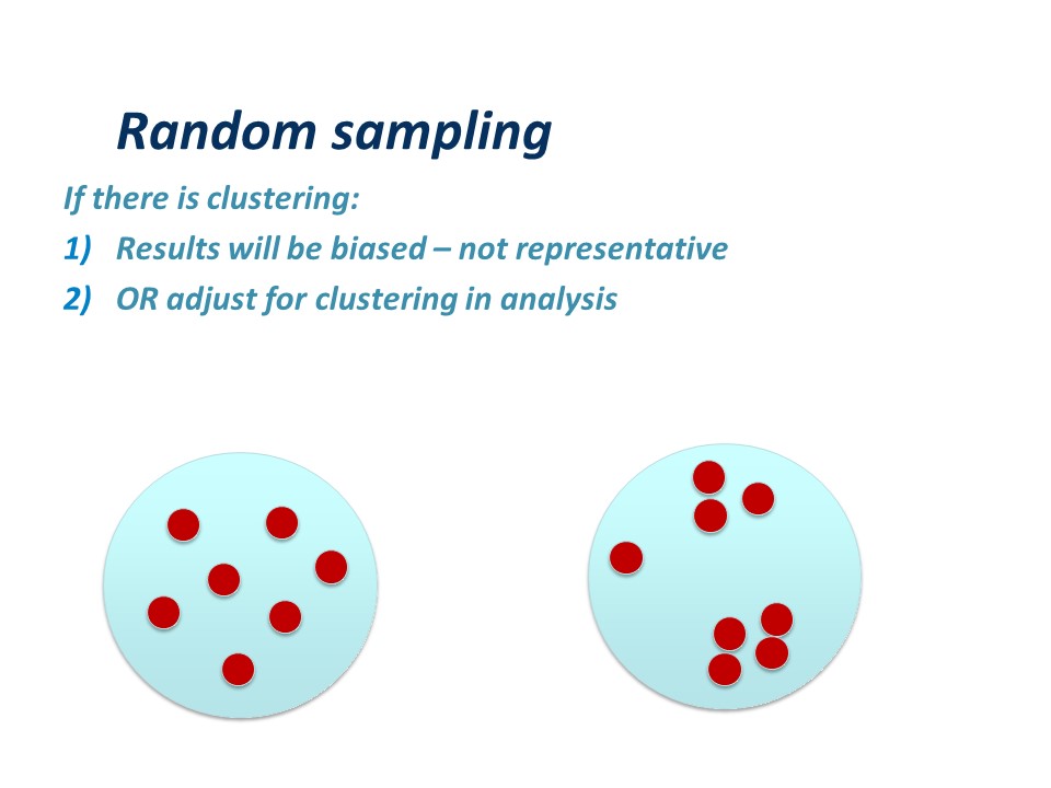
If there is clustering:

Firstly, the results will be biased – because the sample is not representative. You may have selected subjects who are sicker, older, younger, richer, poorer, or different in some other attribute, than the average in the target population. Similar comments apply to any control or reference group.

OR it may be possible to adjust for clustering in analysis – you can use techniques like stratifying your study subjects, or more sophisticated techniques which are outside the scope of this article.

Practical calculation of sample size

Calculating sample size is a whole field of study in itself, but in its basic form is easy. For example, in a cross sectional study, you might wish to measure the proportion of mothers at a particular hospital who deliver by caesarean section. How many mothers do you need to assess for mode of delivery to obtain a reasonably accurate or precise estimate?

You might want to know if term babies born by caesarean section are of ‘normal’ mean birth-weight. You may already know what a normal birth-weight is for Australian born babies.

Probably the most common type of sample size calculation is for a comparison of two means. Most sample size calculations come down to two main types:

Planning your study: sample size questions

How many subjects do I need to show a statistically significant effect (if there is one) of my intervention/risk factor? An alternate way of phrasing this question is ‘how many subjects to I need to show a clinically significant difference of X between two groups?’ – in this latter example you need to decide yourself what you regard as clinically important, for example you may decide that an average in birth-weight between two groups of 100g is clinically significant.

Resources for calculating sample size (or power): online calculators and statistics software

There are many on-line calculators for sample size. Two good ones are:

http://sampsize.sourceforge.net/iface/

www.stat.ubc.ca/~rollin/stats/ssize

Statistical software

STATA (www.stata.com)

SAS (www.sas.com)

SPSS (www.ibm.com/software/au/analytics/spss/products/statistics/)

R (www.r–project.org/)

Commonly used abbreviations

Statistical notation often uses greek letters. Mean is often represented mu (m) and standard as sigma (s). The Type I error is represented as alpha (α) and Type II error as beta (b).

Sample size for prevalence (proportion)

You will need to ‘guess’ the expected prevalence, based perhaps on prior studies or pilot studies, and you need to specify how precise you want your estimates in terms of precision and confidence interval. Typically researchers use 5% precision and 95% confidence interval.

• Prevalence – expected prevalence from literature or previous experience
• Precision – how accurately you wish to measure your prevalence
• Confidence interval – (1 – precision)
• Population size – if unknown estimate will not be adjusted for small population size

We will use a hypothetical example where we wish to estimate the proportion of women in a particular hospital who deliver by caesarean section. We think, from our clinical experience, that around 27% of women delivery by caesarean section. We decide on 5% precision and 95% confidence interval.

In the ‘sampsize’ web calculator (http://sampsize.sourceforge.net/iface/), enter the desired precision, prevalence and confidence level, click on ‘calculate’ and your sample size will come up. The calculation shows that we need to ascertain the mode of delivery in 303 women.

Note: the website specifies that if the prevalence is unknown, enter 50%. This is because measurement of a prevalence of 50% requires the largest sample size, so is a very conservative or ‘safe’ estimate of sample size.

Sample size for two means or two proportions

You might want to calculate a sample size for comparing two means, or two proportions.

For example, you might want to compare the mean fetal weight of infants of women with excessive gestational weight gain with those with acceptable gestational weight gain (this example is adapted from Walsh⁸).

You might want to compare the proportion of women in Australia having caesarean section with the proportion of women in England having caesarean section (adapted from Prosser⁹).

Power and sample size – Type I and Type II error

You need to consider the acceptable level of type 1 or type II error.

The type I or alpha error is often set at 0.05. This is the probability of wrongly accepting a difference if there is really no difference between groups. The ‘alpha’ is the p-value which is the researcher chooses at the beginning of the study, at the design stage. There are many types of statistical tests, all of which result in a ‘test statistic’. For example, a t-test results in a ‘t’ statistic; a chi-square test results in a ‘Chi-square’ statistic; an analysis of variance (ANOVA) results in an ‘F’ statistic.

The p-value is the probability of obtaining a statistic as extreme, or more extreme, than the test statistic, whatever that test statistic might be. In practice, this is the value on the x-axis of a distribution.

For example, the probability of obtaining a t statistic equal to, or more extreme, than plus or minus 2.042, (with 30 degrees of freedom), is 5% or less. The p-value would be 0.05 or less. Look at a table of Student’s t-distribution in any statistics text book to see how this works. Conversely, the ‘critical value’ of t if alpha is set at p-0.05 is plus or minus 2.042.

[Image to be inserted]

The ‘power’ of a study is the chance of detecting a difference between groups, if there is in fact a difference. For biological studies, power is often set at a minimum of 80%, i.e. the study has an 80% chance of detecting a difference between two groups. Power is related to a quantity called ‘beta’. Beta is often set at 0.20 or 20%. Power is calculated as:

power = 1- β

so if beta is set at 0.2, power is correspondingly equal to 0.8 or 80%. This is probability of falsely rejecting the alternate hypothesis, i.e. concluding there is NO difference between groups when there is in fact a difference. An under-powered study might find no difference between groups when in fact there IS a difference.

For example, if we found that estimated fetal weight at 34 weeks was 2681 g compared with 2574 g, and we conclude this is different, but in fact is due to chance (sampling variation), this would be a type I error. At an pre-set alpha of 0.05, there is a 5% chance this will happen.

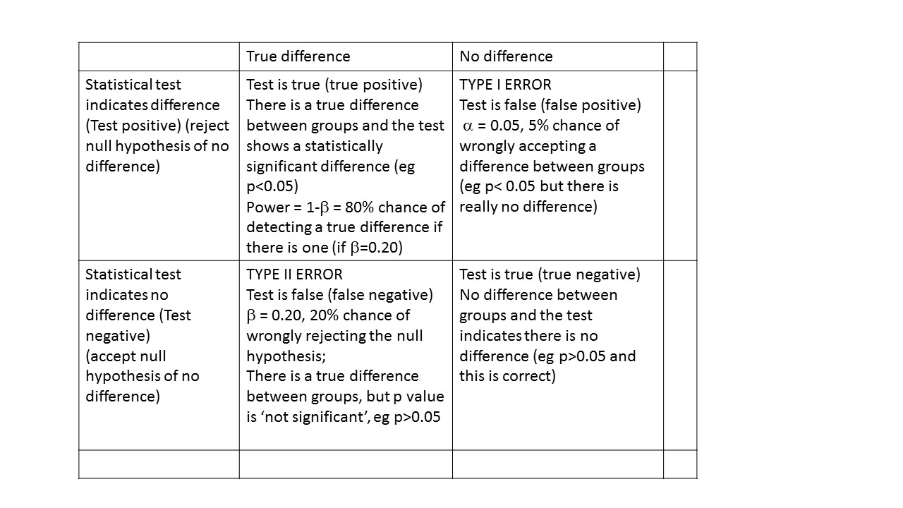
For example, if we found that estimated fetal weight was 2681 g compared 2574 g and we conclude this is not different, but in fact really is different, this would be a type II or beta error.

Power can be interpreted as the probability of finding a difference between groups, if there is one.

Sample size for two means

To calculate the sample size for comparing two means you need:

• Your estimate of mean 1 (μ1) and mean 2 (μ2)
• Your estimate of the standard deviation (SD) of the means
• Your decision about alpha
• Your decision about beta

The difference between means is known as the ‘effect size’. If the means are close together, as in the picture on the left, you will need many subjects. If the means are far apart, with a large effect size, you will not need so many study subjects.

We will use the stat.ubc website (www.stat.ubc.ca/~rollin/stats/ssize) to calculate a sample size to detect the difference between two means. You need to know the power you want your study to have, typically 0.8 (80%), the alpha value or p-value, typically 0.05, and ‘guestimate’ of the pooled standard deviation of your two groups.

Notice you can solve for either power or sample size

• Enter mean one and mean two (often known as mu 1 and mu2)
• Enter values for alpha and power

Click on calculate.

For this example, I used the fetal weights and standard deviations from Jennifer Walsh’s paper.⁸ If mean 1 is 2681 grams, mean 2 is 2574 grams, with standard deviation 345 (standard deviation is often represented by the greek letter sigma), you can see the sample size needed is 164 in each group.

If you want a greater than 80% chance of detecting a difference if there is one, you can increase the power of your study. Similarly if you want a smaller chance of falsely concluding there is a difference when there is really none, you can decrease you alpha value.

Try this with power of 90% and alpha of 0.01!

What was the power of the study actually conducted by Walsh?

Sample size for two proportions

To calculate the sample size for comparing two proportions you need:-

• Your estimate of proportion 1 and proportion 2 (p1 and p2)
• Your decision about alpha
• Your decision about beta

Again using the ‘stat.ubc’ website (www.stat.ubc.ca/~rollin/stats/ssize), we enter our data. For this example, data from Prosser’s paper comparing caesarean rates in Queensland and England⁹ was used. To detect a difference in a proportion of 0.36 compared with 0.25, we need 274 subjects in each group. Note that the ‘real’ report includes many more subjects and analysed many more variables than merely the proportions of women having cs.

Other sample size calculations

There are many more situations where a calculation for power or sample size is required, such as comparing a sample mean to a known population mean, or a sample proportion to a known population proportion.  More complex calculations are required for studies involving ANOVA, crossover studies, regression, and diagnostic tests.

 

1. Everitt BS. The Cambridge Dictionary of Statistics in the Medical Sciences. Cambridge, UK: Cambridge University Press, 1995.
2. CONSORT Website.
3. STROBE Website.
4. Collaboration C. Cochrane Handbook for Systematic Reviews of Interventions, 2011.
5. Altman DG, Bland JM. How to obtain the confidence interval from a P value. BMJ (Clinical research ed.) 2011;343:d2090.
6. Altman DG, Bland JM. Uncertainty and sampling error. BMJ (Clinical research ed.) 2014;349:g7064.
7. Doll H, Carney S. Statistical approaches to uncertainty: P values and confidence intervals unpacked. Equine veterinary journal 2007;39(3):275-6.
8. Walsh JM, McGowan CA, Mahony RM, Foley ME, McAuliffe FM. Obstetric and metabolic implications of excessive gestational weight gain in pregnancy. Obesity (Silver Spring, Md.) 2014;22(7):1594-600.
9. Prosser SJ, Miller YD, Thompson R, Redshaw M. Why ‘down under’ is a cut above: a comparison of rates of and reasons for caesarean section in England and Australia. BMC pregnancy and childbirth 2014;14:149.